
ESN( echo state networks):
针对递归神经网络训练困难以及记忆渐消问题,jaeger 于2001年提出一种新型递归神经网络— — —回声状态网络. ESN网络一经提出便成为学术界的研究热点,并应用到各种不同领域,包括动态模式分类、机器人控制、对象跟踪核运动目标 检 测、 事 件 监 测 等, 尤其是时间序列预测问题.
ESN
ESN 属于RNN的范畴,具有短期记忆的能力。今天将探讨和实验ESN在时间序列问题上的原理。
时间序列数据往往具有高噪声、随机性以及非线性等特点,其建模、分析以及预测问题一直是学术界研究的热点 .一般地讲,为了更加准确地预测时间序列,需要时间序列模型既具有良好的非线性逼近能力,又具有良好的记忆能力 .这对于经典的时间序列建模和分析方法提出极大的挑战 .为了解决非线性时间序列预测问题,支持向量机、神经网络等人工智能方法被引入到时间序列分析领域.
ESN结构
相对于传统神经网络结构ESN所学习的并不是神经元的权重,二是神经元之间的链接。
回声状态状态网络作为一种新型的递归神经网络,无论是建模还是学习算法,都已经与传统的递归神经网络差别很大。
比较直观的结构如下: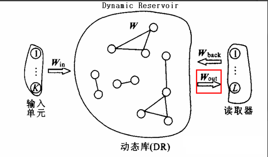
ESN网络特点:
假设系统具有M个输入单元,N个内部处理单元(Processing elements PEs),即N个内部神经元,同时具有L个输出单元,输入单元、内部状态、以及输出单元n时刻的值分别为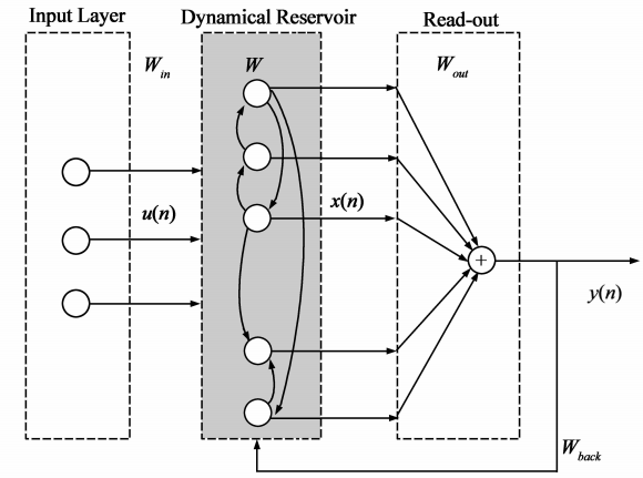
$$u\left( n \right) =\left[ u_1\left( n \right) ,…,u_M\left( n \right) \right] ^T$$
$$x\left( n \right) =\left[ x_1\left( n \right) ,…,x_N\left( n \right) \right] ^T$$
$$y\left( n \right) =\left[ y_1\left( n \right) ,…,y_L\left( n \right) \right] ^T$$
其中,$u\left( n \right) \in R^{K\times 1}$ , $x\left( n \right) \in R^{N\times 1}$ , $y\left( n \right) \in R^{L\times 1}$
从结构上讲,ESNs是一种特殊类型的神经网络,其基本思想是使用大规模随机连接的递归网络,取代经典神经网络中的中间层,从而简化网络的训练过程,回声状态网络的状态方程为:
$$x\left( n+1 \right) =f\left( Wx\left( n \right) +W^{in}u\left( n \right) +W^{back}y\left( n \right) \right) $$
$$
y\left( n+1 \right) =f_{out}\left( W^{out}\left[ x\left( n+1 \right) ,u\left( n+1 \right) ,y\left( n \right) \right] +b^{out} \right)$$
其中,$W\in R^{N\times N}$ , $W^{in}\in R^{N\times K}$ , $W^{back}\in R^{N\times L}$ , $W^{out}\in R^{\left( L+K+N \right) \times L}$
f为激活函数,一般为双曲正切函数。
其中W, $W^{in}$ , $W^{back}$ 分别表示状态变量、输入和输出对状态变量的连接权矩阵;$W^{out}$ 表示储备池、输入和输出对于输出的连接权矩阵,$b^{out}$ 表示输出的偏置项或者可以代表噪声,表示内部神经元激活函数,在网络训练过程中,连接到储备池的连接权矩阵 W, $W^{in}$ , $W^{back}$ 随机产生,一经产生就固定不变.而连接到输出的连接权矩阵 $W^{out}$ 需要通过训练得到,因为状态变量、输入和输出与输出之间是线性关系,所以通常这些连接权只需通过求解线性回归问题得到。
ESN的训练
ESNs的训练过程就是根据给定的训练样本 $u\left( n \right) =\left[ u_1\left( n \right) ,…,u_M\left( n \right) \right] ^T$ ,确定系统输出连接权矩阵
$W^{out}$的过程 .
ESNs的训练分为两个过程: 采样过程和权值计算过程
采样过程
采样阶段首先任意选定网络的初始状态,但是通常情况下选取网络的初始状态为0,即 $x(0)=0$ ,训练样本$u\left( n \right) =\left[ u_1\left( n \right) ,…,u_M\left( n \right) \right] ^T$ 经过输入连接权矩阵 $W^{in}$ 被加入到储备池中, 按照方程,依次完成系统状态和输出珋 $y(n)$ 的计算与收集 . 为了计算输出连接权矩阵,需要从某一时刻 m 开始收集(采样)内部状态变量,并以向量 $x\left( n \right) =\left[ x_1\left( n \right) ,…,x_N\left( n \right) \right] ^T$ 为行构成矩阵,同时相应的样本数据 y(n)也被收集,并构成一个列向量 $B\in R^{\left( p-m+1 \right) \times N}$ ,同时相应的样本数据y(n)也被收集,并构成 $T\in R^{\left( p-m+1 \right) \times L}$
权值计算
权值计算就是根据在采样阶段收集到系统状态矩阵和样本数据,计算输出连接权 $W^{out}$ . 因为状态变量 $x(n)$ 和系统输出 $y(n)$ 之间是线性关系,而需要实现的目标是利用网络实际输出逼近期望输出 :
$$y\left( n \right) \approx \hat{y}\left( n \right) =\sum_{i=1}^L{w_{i}^{out}x_i\left( n \right)}$$
所以损失函数为:
$$\underset{w_{i}^{out}}{\min}\frac{1}{p-m+1}\sum_{n=m}^P{\left( y\left( n \right) -\sum_{i=1}^L{w_{i}^{out}x_i\left( n \right)} \right) ^2}$$
所以其训练过程可以用于计算:
$$W^{out}=B^{-1}T $$
实验
实验代码:https://github.com/unsky/esn-rmlp
主程序
esn_main.m
训练数据准备
seq_gen_esn 用于产生3000个训练数据
网络训练
esn_train用于网络训练求得 $W^{out}$
|
|
测试结果
esn_test
实验结果
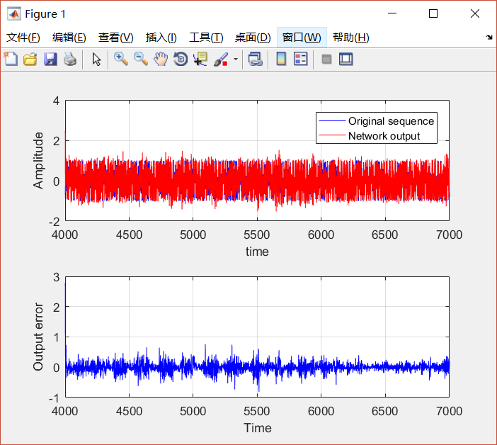
从错误率可以看出,ESNs的误差率可以接受。。